Tag: technology

  • Build Your First MCP Server in 20 Minutes

    Build Your First MCP Server in 20 Minutes

    In the [last post](/mcp-architecture), we went deep on how MCP works—the protocol handshake, JSON-RPC messages, and transport layers. Now it’s time to get our hands dirty.

    By the end of this post, you’ll have a working MCP server running on your machine. We’re going with Python because it’s the fastest path to “holy crap, this actually works.”

    No frameworks. No boilerplate hell. Just a single file that turns your code into something Claude can actually use.

    What We’re Building

    We’re creating a Notes Server—a simple tool that lets Claude:

    • Save notes with a title and content
    • List all saved notes
    • Read a specific note by title
    • Search notes by keyword
    • Delete notes

    It’s simple enough to build in 20 minutes, but real enough to teach you everything you need to know about MCP.

    Why notes instead of another weather API example? Because notes are stateful. They persist between calls. That’s where MCP starts to get interesting.

    Prerequisites

    Before we start, make sure you have:

    • Python 3.10+ installed
    • Claude Desktop or another MCP-compatible client
    • About 20 minutes of uninterrupted time

    That’s it. No complex setup, no cloud accounts.

    Step 1: Set Up the Project

    First, let’s create a project directory and install the MCP SDK. We’re using uv because it’s fast and handles virtual environments cleanly:

    # Install uv if you haven’t already
    # Windows (PowerShell)
    irm https://astral.sh/uv/install.ps1 | iex

    # macOS/Linux
    curl -LsSf https://astral.sh/uv/install.sh | sh

    Now set up the project:

    # Create project directory
    uv init mcp-notes-server
    cd mcp-notes-server

    # Create and activate virtual environment
    uv venv
    # Windows
    .venv\Scripts\activate
    # macOS/Linux
    source .venv/bin/activate

    # Install MCP SDK
    uv add “mcp[cli]”

    # Create our server file
    # Windows
    type nul > notes_server.py
    # macOS/Linux
    touch notes_server.py

    Your project structure should look like this:

    mcp-notes-server/
    ├── .venv/
    ├── pyproject.toml
    └── notes_server.py

    Step 2: The Minimal Server

    Let’s start with the absolute minimum—a server that does nothing but exist. Open notes_server.py and add:

    from mcp.server.fastmcp import FastMCP

    # Initialize the MCP server with a name
    mcp = FastMCP(“notes”)

    if __name__ == “__main__”:
        mcp.run(transport=”stdio”)

    That’s a valid MCP server. It doesn’t do anything useful yet, but it speaks the protocol.

    The FastMCP class handles all the protocol machinery—handshakes, message routing, capability negotiation. We just need to tell it what tools to expose.

    Step 3: Add State (The Notes Storage)

    Before we add tools, we need somewhere to store notes. For simplicity, we’ll use an in-memory dictionary. In production, you’d use a database.

    from mcp.server.fastmcp import FastMCP
    from datetime import datetime

    # Initialize the MCP server
    mcp = FastMCP(“notes”)

    # In-memory storage for notes
    # Key: title (str), Value: dict with content and metadata
    notes_db: dict[str, dict] = {}

    Step 4: Add Your First Tool

    Now the fun part. Let’s add a tool that saves notes:

    @mcp.tool()
    def save_note(title: str, content: str) -> str:
        “””
        Save a note with a title and content.
       
        Args:
            title: The title of the note (used as identifier)
            content: The content of the note
        “””
        notes_db[title] = {
            “content”: content,
            “created_at”: datetime.now().isoformat(),
            “updated_at”: datetime.now().isoformat()
        }
        return f”Note ‘{title}’ saved successfully.”

    That’s it. One decorator. The @mcp.tool() decorator does several things:

    1. Registers the function as an MCP tool

    2. Generates the input schema from type hints (title: str, content: str)

    3. Extracts the description from the docstring

    4. Handles the JSON-RPC wrapper automatically

    When Claude calls tools/list, it will see something like:

    {
      “name”: “save_note”,
      “description”: “Save a note with a title and content.”,
      “inputSchema”: {
        “type”: “object”,
        “properties”: {
          “title”: {“type”: “string”, “description”: “The title of the note (used as identifier)”},
          “content”: {“type”: “string”, “description”: “The content of the note”}
        },
        “required”: [“title”, “content”]
      }
    }

    The SDK parsed your docstring and type hints to build that schema. No manual JSON schema writing required.

    Step 5: Complete the Tools

    Let’s add the remaining tools:

    @mcp.tool()
    def list_notes() -> str:
        “””
        List all saved notes with their titles and creation dates.
        “””
        if not notes_db:
            return “No notes saved yet.”
       
        note_list = []
        for title, data in notes_db.items():
            note_list.append(f”- {title} (created: {data[‘created_at’][:10]})”)
       
        return “Saved notes:\n” + “\n”.join(note_list)


    @mcp.tool()
    def read_note(title: str) -> str:
        “””
        Read the content of a specific note.
       
        Args:
            title: The title of the note to read
        “””
        if title not in notes_db:
            return f”Note ‘{title}’ not found.”
       
        note = notes_db[title]
        return f”””Title: {title}
    Created: {note[‘created_at’]}
    Updated: {note[‘updated_at’]}

    {note[‘content’]}”””


    @mcp.tool()
    def search_notes(keyword: str) -> str:
        “””
        Search notes by keyword in title or content.
       
        Args:
            keyword: The keyword to search for (case-insensitive)
        “””
        if not notes_db:
            return “No notes to search.”
       
        keyword_lower = keyword.lower()
        matches = []
       
        for title, data in notes_db.items():
            if keyword_lower in title.lower() or keyword_lower in data[“content”].lower():
                matches.append(title)
       
        if not matches:
            return f”No notes found containing ‘{keyword}’.”
       
        return f”Notes matching ‘{keyword}’:\n” + “\n”.join(f”- {title}” for title in matches)


    @mcp.tool()
    def delete_note(title: str) -> str:
        “””
        Delete a note by title.
       
        Args:
            title: The title of the note to delete
        “””
        if title not in notes_db:
            return f”Note ‘{title}’ not found.”
       
        del notes_db[title]
        return f”Note ‘{title}’ deleted.”

    Step 6: The Complete Server

    Here’s the full notes_server.py:

    “””
    MCP Notes Server
    A simple server that lets AI assistants manage notes.
    “””

    from mcp.server.fastmcp import FastMCP
    from datetime import datetime

    # Initialize the MCP server
    mcp = FastMCP(“notes”)

    # In-memory storage for notes
    notes_db: dict[str, dict] = {}


    @mcp.tool()
    def save_note(title: str, content: str) -> str:
        “””
        Save a note with a title and content.
       
        Args:
            title: The title of the note (used as identifier)
            content: The content of the note
        “””
        notes_db[title] = {
            “content”: content,
            “created_at”: datetime.now().isoformat(),
            “updated_at”: datetime.now().isoformat()
        }
        return f”Note ‘{title}’ saved successfully.”


    @mcp.tool()
    def list_notes() -> str:
        “””
        List all saved notes with their titles and creation dates.
        “””
        if not notes_db:
            return “No notes saved yet.”
       
        note_list = []
        for title, data in notes_db.items():
            note_list.append(f”- {title} (created: {data[‘created_at’][:10]})”)
       
        return “Saved notes:\n” + “\n”.join(note_list)


    @mcp.tool()
    def read_note(title: str) -> str:
        “””
        Read the content of a specific note.
       
        Args:
            title: The title of the note to read
        “””
        if title not in notes_db:
            return f”Note ‘{title}’ not found.”
       
        note = notes_db[title]
        return f”””Title: {title}
    Created: {note[‘created_at’]}
    Updated: {note[‘updated_at’]}

    {note[‘content’]}”””


    @mcp.tool()
    def search_notes(keyword: str) -> str:
        “””
        Search notes by keyword in title or content.
       
        Args:
            keyword: The keyword to search for (case-insensitive)
        “””
        if not notes_db:
            return “No notes to search.”
       
        keyword_lower = keyword.lower()
        matches = []
       
        for title, data in notes_db.items():
            if keyword_lower in title.lower() or keyword_lower in data[“content”].lower():
                matches.append(title)
       
        if not matches:
            return f”No notes found containing ‘{keyword}’.”
       
        return f”Notes matching ‘{keyword}’:\n” + “\n”.join(f”- {title}” for title in matches)


    @mcp.tool()
    def delete_note(title: str) -> str:
        “””
        Delete a note by title.
       
        Args:
            title: The title of the note to delete
        “””
        if title not in notes_db:
            return f”Note ‘{title}’ not found.”
       
        del notes_db[title]
        return f”Note ‘{title}’ deleted.”


    if __name__ == “__main__”:
        mcp.run(transport=”stdio”)

    That’s under 110 lines of code. Five tools. A complete MCP server.

    Step 7: Test the Server

    Before connecting to Claude, let’s verify the server works. The MCP SDK includes a development server:

    uv run mcp dev notes_server.py

    This starts an interactive inspector where you can test your tools manually. You’ll see all five tools listed, and you can call them with different inputs.

    Step 8: Connect to Claude Desktop

    Now let’s connect our server to Claude Desktop.

    Open Claude Desktop’s configuration file:

    • Windows: %APPDATA%\Claude\claude_desktop_config.json
    • macOS: ~/Library/Application Support/Claude/claude_desktop_config.json

    Add your server configuration:

    {
      “mcpServers”: {
        “notes”: {
          “command”: “uv”,
          “args”: [
            “–directory”,
            “C:/path/to/mcp-notes-server”,
            “run”,
            “notes_server.py”
          ]
        }
      }
    }

    Important: Replace C:/path/to/mcp-notes-server with the actual path to your project directory. Use forward slashes even on Windows.

    Restart Claude Desktop. You should now see a hammer icon (🔨) indicating MCP tools are available.

    Step 9: Use It

    Open Claude Desktop and try these prompts:

    “Save a note called ‘Meeting Notes’ with the content ‘Discussed Q1 roadmap. Action items: review budget, schedule follow-up.’”

    Claude will call your save_note tool and confirm the save.

    “What notes do I have?”

    Claude calls list_notes and shows your saved notes.

    “Search my notes for ‘budget’”

    Claude calls search_notes and finds the matching note.

    It works. Your Python functions are now accessible to an LLM. That’s MCP in action.

    What Just Happened?

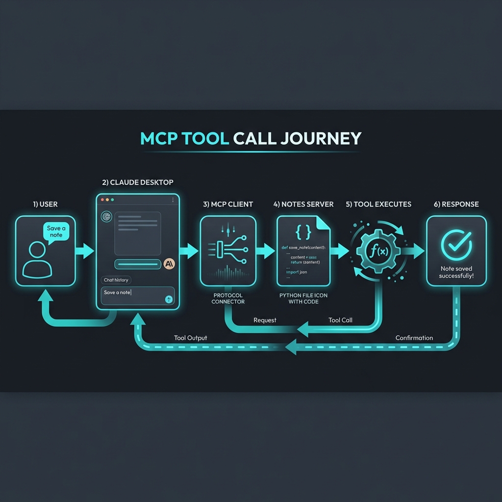
    Let’s break down the flow:

    1. Claude Desktop spawns your server as a subprocess

    2. Protocol handshake happens automatically (remember Blog 2?)

    3. Claude queries tools/list and discovers your five tools

    4. When you ask about notes, Claude decides which tool to call

    5. Your Python function runs, returns a string

    6. Claude incorporates the result into its response

    You didn’t write any JSON-RPC handlers. No WebSocket code. No API routes. The SDK handled all of that.

    Adding a Resource (Bonus)

    Tools are great for actions, but what about data that should be pre-loaded into Claude’s context? That’s what Resources are for.

    Let’s add a Resource that exposes all notes as a single document:

    @mcp.resource(“notes://all”)
    def get_all_notes() -> str:
        “””
        Get all notes as a single document.
        “””
        if not notes_db:
            return “No notes available.”
       
        output = []
        for title, data in notes_db.items():
            output.append(f”## {title}\n\n{data[‘content’]}\n”)
       
        return “\n—\n”.join(output)

    Now Claude can read notes://all to get context about all your notes at once, without needing to call list_notes and read_note multiple times.

    Common Gotchas

    Print statements break stdio transport

    If you add print() statements for debugging, they’ll corrupt the JSON-RPC stream. Stdio uses stdout for protocol messages—your prints hijack that.

    Use logging instead:

    import logging
    logging.basicConfig(level=logging.DEBUG)
    logger = logging.getLogger(__name__)

    # This is fine
    logger.debug(“Processing request…”)

    Type hints matter

    The SDK generates input schemas from your type hints. If you write:

    def save_note(title, content):  # No type hints

    The schema won’t know what types to expect. Always annotate your parameters.

    Docstrings are your API docs

    The docstring becomes the tool description that Claude sees. Write clear descriptions—the LLM uses them to decide when to call your tool.

    What’s Next?

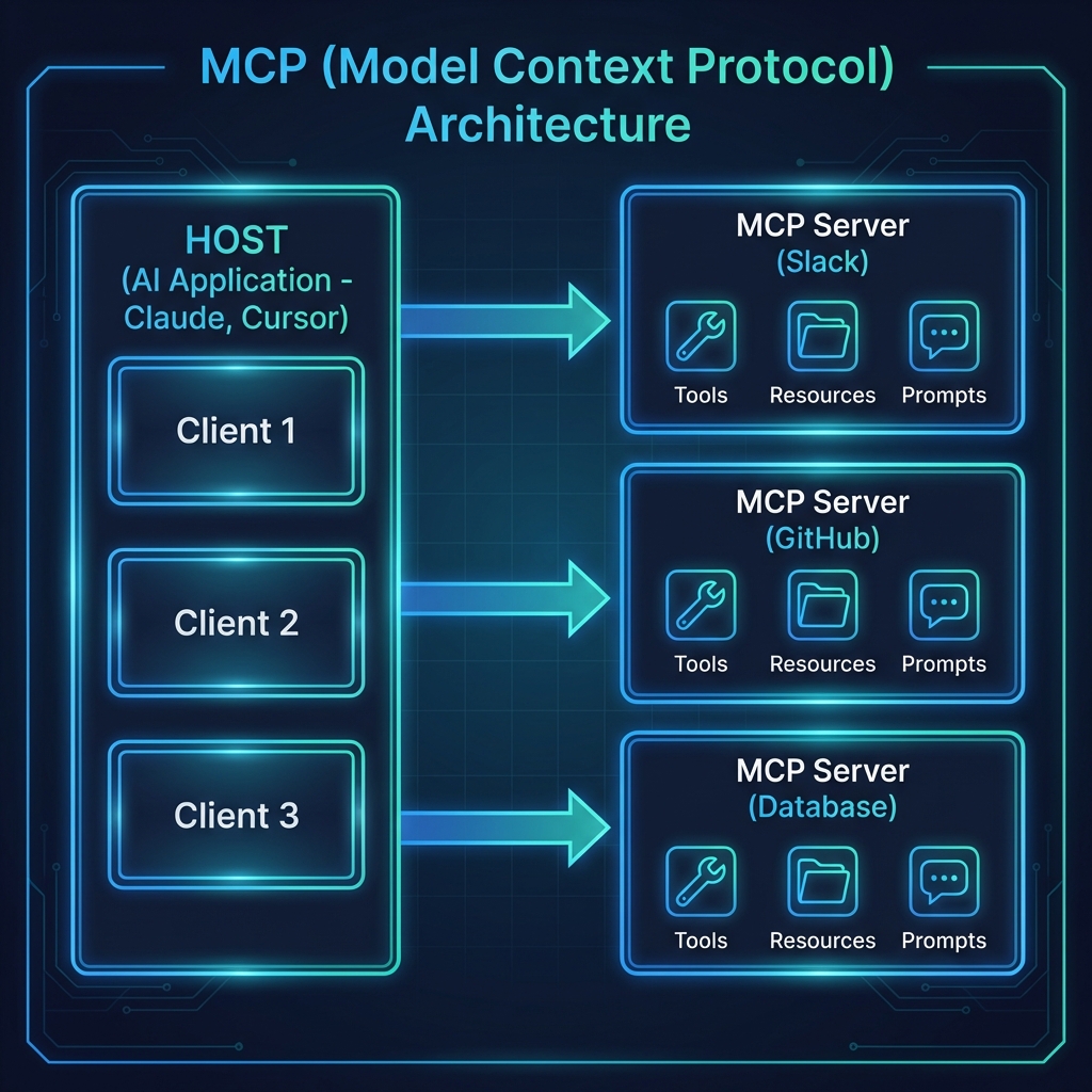
    You’ve built your first MCP server. In Blog 4, we’ll look at real-world patterns—how companies are using MCP to connect everything from Slack to databases to proprietary internal systems.

    The notes server is a toy. But the pattern is universal: expose functions as tools, expose data as resources, let the LLM orchestrate.

    This is the third post in a series on MCP. Here’s what’s coming:

    1. ✅ This Post: Why MCP matters

    2. ✅ Blog 2: Under the Hood—deep dive into architecture, transports, and the protocol spec

    3. ✅ Blog 3: Build Your First MCP Server in 20 minutes (Python/TypeScript)

    4. Blog 4: MCP in the Wild—real-world patterns and use cases

    5. Blog 5: Security, OAuth, and the agentic future

    For the official MCP examples, see the [quickstart-resources repo](https://github.com/modelcontextprotocol/quickstart-resources) and the [SDK examples](https://github.com/modelcontextprotocol/python-sdk/tree/main/examples).

  • MCP: The Future of AI Integration Standards

    MCP: The Future of AI Integration Standards

    We’ve all been there. You spend three days writing a custom connector to hook your AI assistant into Salesforce. It works. You celebrate. A week later, the API changes, and it breaks. Meanwhile, your colleague is doing the exact same thing for Slack. And another team is doing it for the internal CRM.

    This is the Integration Tax—the endless cycle of building, maintaining, and rebuilding connectors every time you want an AI model to actually do something useful.

    In November 2024, Anthropic decided to stop paying this tax. They released the Model Context Protocol (MCP)—an open standard that’s quickly becoming what USB-C did for charging cables.

    The N×M Problem

    Before we talk about the solution, let’s be clear about the problem.

    Say you have 5 AI tools (Claude, ChatGPT, Cursor, your internal agent, etc.) and 10 data sources (Slack, GitHub, Postgres, Google Drive, your proprietary API…). Without a standard, you need 50 custom integrations. Every combination needs its own connector.

    Now scale that. Add a new model? Build 10 more connectors. Add a new data source? Build 5 more. The math gets ugly fast.

    This isn’t a hypothetical. It’s what enterprises are living through right now. Anthropic called it being “trapped behind information silos and legacy systems.” I call it expensive, boring, and fundamentally unscalable.

    Enter MCP: The USB-C Analogy

    Remember the drawer full of proprietary chargers? Nokia had one plug. Samsung had another. Apple had three different ones depending on the year. It was chaos.

    Then USB-C happened. One port. Universal compatibility. The drawer got emptier.

    MCP is the USB-C moment for AI agents.

    Instead of N×M integrations, you get N + M. Each AI tool implements the MCP client once. Each data source implements the MCP server once. They all just… work together.

    And here’s the kicker: this isn’t an Anthropic-only play. OpenAI and Google have signaled adoption. The open-source community is building servers for everything from Notion to Kubernetes. It’s not a walled garden—it’s a public utility.

    How It Works (The 30-Second Version)

    Picture: [MCP Architecture]

    MCP has three actors:

    ComponentRole
    HostThe AI application (Claude Desktop, Cursor, your custom agent)
    ClientThe protocol connector inside the Host—translates requests
    ServerThe external capability (Slack, GitHub, your Postgres database)

    When you ask Claude to “check my calendar and book a flight,” here’s what happens:

    1. The Host (Claude) asks its Client: “What servers are available?”

    2. The Client checks connected MCP Servers and finds a Calendar server and a Travel server.

    3. The Host uses Tools from those servers to execute actions.

    The Host doesn’t need to know how the Calendar server works. It just asks “what can you do?” and the server responds with a list of capabilities.

    The Three Primitives

    MCP servers expose three types of capabilities:

    PrimitiveWhat It DoesExample
    ToolsExecute actionssearchFlights(), sendEmail(), queryDatabase()
    ResourcesProvide datafile:///docs/report.pdf, calendar://events/2024
    PromptsOffer interaction templatesA plan-vacation workflow with structured inputs

    Tools are the “do this” commands—API calls, database queries, file operations.

    Resources are the “read this” data sources—files, logs, records, anything with a URI.

    Prompts are pre-packaged workflows that guide the AI through multi-step tasks.

    A single MCP server might expose all three. A filesystem server gives you Tools to create files, Resources to read them, and maybe a Prompt for “organize this folder.”

    The Ecosystem Is Already Here

    This isn’t vaporware. The ecosystem is moving fast.

    Early Adopters:

    • Block (formerly Square) is building agentic systems with MCP
    • Apollo has integrated it into their workflows
    • Zed, Replit, Codeium, Sourcegraph—the AI coding tools are all in

    SDKs in 10 Languages:

    TypeScript, Python, Go, Kotlin, Swift, Java, C#, Ruby, Rust, PHP

    100+ Third-Party Integrations:

    Slack, GitHub, Notion, Postgres, Google Drive, Figma, Salesforce, Sentry, Puppeteer… the list keeps growing.

    There’s even an [MCP Registry](https://registry.modelcontextprotocol.io/) where you can browse published servers.

    Why Should You Care?

    If you’re a developer:

    Build one MCP server for your internal API. Suddenly, every MCP-compatible AI tool can use it—Claude, Cursor, whatever comes next. No more rewriting connectors.

    If you’re running a company:

    MCP means no vendor lock-in. If you switch from Claude to GPT-5 to Gemini, your data layer stays the same. The Integration Tax drops to near-zero.

    If you’re a user:

    Your AI assistant finally has context. It can read your files, check your calendar, and take actions—without you copy-pasting information between apps.

    What’s Next

    This is the first post in a series on MCP. Here’s what’s coming:

    1. ✅ This Post: Why MCP matters

    2. Blog 2: Under the Hood—deep dive into architecture, transports, and the protocol spec

    3. Blog 3: Build Your First MCP Server in 20 minutes (Python/TypeScript)

    4. Blog 4: MCP in the Wild—real-world patterns and use cases

    5. Blog 5: Security, OAuth, and the agentic future

    The Integration Tax era is ending. The question isn’t if MCP becomes the standard—it’s how fast you get on board.

    Want to explore? Start at [modelcontextprotocol.io](https://modelcontextprotocol.io) or browse the [MCP Registry](https://registry.modelcontextprotocol.io/).

    – Satyajeet Shukla

    AI Strategist & Solutions Architect

  • Beyond the Binary: Monoliths, Event-Driven Systems, and the Hybrid Future

    Beyond the Binary: Monoliths, Event-Driven Systems, and the Hybrid Future

    In software engineering, architectural discussions often devolve into a binary choice: the “legacy” Monolith versus the “modern” Microservices. This dichotomy is not only false but dangerous. It forces teams to choose between the operational simplicity of a single unit and the decoupled scalability of distributed systems, often ignoring a vast middle ground.

    Recently, the rise of API-driven Event-Based Architectures (EDA) has added a third dimension, promising reactive, real-time systems. But for a technical leader or a systems architect, the question isn’t “which is best?” but “which constraints am I optimising for?”

    This article explores the trade-offs between Monolithic and Event-Driven systems and makes a case for the pragmatic middle ground: the Hybrid approach.

    1. The Monolith: Alive and Kicking

    The term “Monolith” often conjures images of unmaintainable “Big Ball of Mud” codebases. However, a well-designed Modular Monolith is a legitimate architectural choice for 90% of use cases.

    The Strengths

    •   Transactional Integrity (ACID): The single biggest advantage of a monolith is the ability to run a complex business process (e.g., “Place Order”) within a single database transaction. If any part fails, the whole operation rolls back. In distributed systems, this simple guarantee is replaced by complex Sagas or two-phase commits.
    •   Operational Simplicity: One deployment pipeline, one monitoring dashboard, one database to back up. The cognitive load on the ops team is significantly lower.
    •   Zero-Latency Communication: Function calls are orders of magnitude faster than network calls. You don’t need to worry about serialization overhead, network partitions, or retries.

    Limiters

    The monolith hits a wall when team scale outpaces code modularity. When 50 developers are merging into the same repo, the merge conflicts and slow CI/CD pipelines become the bottleneck.

    2. API-Driven Event-Based Architectures

    In this model, services don’t just “call” each other via HTTP; they emit “events” (facts about what just happened) to a broker (Kafka, RabbitMQ, EventBridge). Other services subscribe to these events and react.

    The Strengths

    •   True Decoupling: The OrderService doesn’t know the EmailService exists. It just screams “OrderPlaced” into the void. This allows you to plug in new functionality (e.g., a “FraudDetection” service) without touching the core flow.
    •   Asynchronous Resilience: If the InventoryService is down, the OrderService can still accept orders. The events will just sit in the queue until the consumer recovers.
    •   Scale Asymmetry: An image processing service might need 100x more CPU than the user profile service. You can scale them independently without over-provisioning the rest of the system.

    The Tax

    The cost of this power is complexity. You now live in a world of eventual consistency. A user might place an order but not see it in their history for 2 seconds. Debugging a flow that jumps across 5 services via inconsistent message queues requires sophisticated observability (Distributed Tracing) and mature DevOps practices.

    3. The Hybrid Approach: The “Citadel” and Modular Monoliths

    It is rarely an all-or-nothing decision. The most successful systems often employ a hybrid strategy, famously described by some as the Citadel Pattern or the Strangler Fig.

    Pattern A: The Modular Monolith (Internal EDA)

    You build a single deployable unit, but internally, you enforce strict boundaries.

    •   Internal Events: Instead of Module A calling Module B’s class directly, you can use an in-memory event bus. When a user registers, the User Module publishes a domain event. The Notification Module subscribes to it.
    •   Why?: This gives you the decoupling benefits of EDA (code isolation) without the operational tax of distributed systems (network failures, serialization).

    Pattern B: The Citadel (Monolith + Satellites)

    Keep your core, complex business domain (e.g., the billing engine or policy ledger) in a Monolith. This domain likely benefits from ACID transactions and complex data joins.

    •   Offload peripheral or high-scale volatility to microservices.
    •   Example: A core Banking Monolith handles the ledger. However, the “PDF Statement Generation” is an external microservice because it is CPU intensive and stateless. The “Mobile API Adapter” is a separate service to allow for rapid iteration on UI needs without risking the core bank.

    4. The Cost Dimension: Infrastructure & People

    Cost is often the silent killer in architectural decisions. It’s not just about the AWS bill; it’s about the Total Cost of Ownership (TCO).

    Infrastructure Costs

    •   Monolith: generally cheaper at low-to-medium scale. You pay for fixed compute (e.g., 2 EC2 instances). You save on data transfer costs because communication is in-memory. However, scaling is inefficient: if one module needs more RAM, you have to upgrade the entire server.
    •   Event-Driven/Microservices: The “Cloud Tax” is real. You pay for:
    •   Managed Services: Kafka (MSK) or RabbitMQ clusters are not cheap to run or cheap to rent.
    •   Data Transfer: Every event crossing an Availability Zone (AZ) or Region boundary incurs a cost.
    •   Base Overhead: Running 50 containers requires more base CPU/RAM overhead than running 1 container with 50 modules.
    •   Savings: You only save money at massive scale, where granular scaling (generating 1000 tiny instances for just the billing service) outweighs the overhead tax.

    Organizational Costs (Engineering Salary)

    •   Monolith: Lower. Generalist developers can contribute easily. Operations require fewer specialists.
    •   Event-Driven: Higher. You need strict platform engineering, SREs to manage the service mesh/brokers, and developers who understand distributed tracing and idempotency.

    Decision Framework: When to Prefer Which?

    Don’t follow the hype. Follow the constraints.

    ConstraintPrefer MonolithPrefer Event-Driven/Microservices
    Team SizeSmall (< 20 engineers), tight communication.Large, multiple independent squads (2-pizza teams).
    Domain ComplexityHigh complexity, deep coupling, needs strict consistency.Clearly defined sub-domains (e.g., Shipping is distinct from Billing).
    Traffic PatternsUniform scale requirement.Asymmetrical scale (one feature needs massive scale).
    ConsistencyStrong (ACID) is non-negotiable.Eventual consistency is acceptable.
    Cost SensitivityBootstrapped/Low Budget. Optimizes for low operational overhead.High Budget/Enterprise. Willing to pay premium for high availability and granular scale.

    Conclusion

    Hybrid approaches allow you to “architect for the team you have, not the team you want.” Start with a Modular Monolith. Use internal events to decouple your code. Only when a specific module needs independent scaling or has a distinct release cycle should you carve it out into a separate service.

    By treating architecture as a dial rather than a switch, you avoid the complexity tax until you actually need the power it buys you.

    -Satyjeet Shukla

    AI Strategist & Solutions Architect

  • Kafka Streams Rebalance Troubleshooting

    Kafka Streams Rebalance Troubleshooting

    Confluent Kafka 2.x

    Problem Statement

    ComponentConfiguration
    Topic Partitions32
    Consumer TypeKafka Streams (intermediate topic)
    DeploymentStatefulSet with 8 replicas
    Stream Threads2 per replica (16 total)
    Expected Distribution2 partitions per thread

    Issue: 10 partitions with lag are all assigned to a single client while 7 other clients sit idle. Deleting pods or scaling down doesn’t trigger proper rebalancing—the same pod keeps picking up the load.

    Root Cause Analysis

    Why This Happens

    Sticky Partition Assignor: Kafka Streams uses StreamsPartitionAssignor which is sticky by design. It tries to maintain partition assignments across rebalances to minimize state migration.

    StatefulSet Predictable Naming: Pod names are predictable (app-0, app-1, etc.). The client.id remains the same after pod restart. Kafka treats it as the “same” consumer returning.

    State Store Affinity: For stateful operations, the assignor prefers keeping partitions with consumers that already have the state.

    Static Group Membership: If group.instance.id is configured, the broker remembers assignments even after pod restart.

    Solutions

    1. Check for Static Group Membership

    If you are using static group membership, the broker remembers the assignment even after pod restart.

    # Check if this is set in your Kafka Streams config

    group.instance.id=<some-static-id>

    Fix: Remove it entirely or make it dynamic.

    2. Proper Scale Down/Up with Timeout Wait

    The key is waiting for session.timeout.ms to expire (default: 45 seconds in Kafka Streams 2.x).

    kubectl scale statefulset <statefulset-name> –replicas=0

    sleep 60

    kubectl scale statefulset <statefulset-name> –replicas=8

    3. Delete the Consumer Group

    ⚠️ Warning: Only do this when ALL consumers are stopped.

    # Scale down to 0

    kubectl scale statefulset <statefulset-name> –replicas=0

    # Verify no active members

    kafka-consumer-groups –bootstrap-server <broker:port> –group <application.id> –describe –members

    # Delete the consumer group

    kafka-consumer-groups –bootstrap-server <broker:port> –group <application.id> –delete

    # Scale back up

    kubectl scale statefulset <statefulset-name> –replicas=8

    4. Reset Consumer Group Offsets

    Resets assignments while preserving current offsets:

    kafka-consumer-groups –bootstrap-server <broker:port> –group <application.id> –reset-offsets –to-current –all-topics –execute

    5. Force New Client IDs

    Modify your StatefulSet to include a random/timestamp suffix in client ID.

    6. Change Application ID (Nuclear Option)

    Creates a completely new consumer group:

    props.put(StreamsConfig.APPLICATION_ID_CONFIG, “my-app-v2”);

    ⚠️ Warning: This will create a new consumer group and reprocess from the beginning.

    7. Enable Cooperative Rebalancing (Kafka 2.4+)

    For Kafka Streams 2.4 and later, cooperative rebalancing provides incremental rebalancing.

    props.put(StreamsConfig.UPGRADE_FROM_CONFIG, “2.3”);

    8. Tune Partition Assignment

    Adjust these configurations for better distribution:

    ACCEPTABLE_RECOVERY_LAG_CONFIG = 10000L

    NUM_STANDBY_REPLICAS_CONFIG = 1

    PROBING_REBALANCE_INTERVAL_MS_CONFIG = 600000L

    Diagnostic Commands

    Check Current Consumer Group Status

    kafka-consumer-groups –bootstrap-server <broker:port> –group <application.id> –describe

    Check Member Assignments (Verbose)

    kafka-consumer-groups –bootstrap-server <broker:port> –group <application.id> –describe –members –verbose

    Monitor Lag

    kafka-consumer-groups –bootstrap-server <broker:port> –group <application.id> –describe | grep -v “^$” | sort -t” ” -k5 -n -r

    Recommended Fix Sequence

    1. Check current state with –describe –members –verbose

    2. Scale down completely: kubectl scale statefulset <name> –replicas=0

    3. Wait for session timeout (60+ seconds): sleep 90

    4. Verify group is empty

    5. Delete consumer group (if still exists)

    6. Scale back up: kubectl scale statefulset <name> –replicas=8

    7. Verify new distribution after 30 seconds

    Prevention (Long-term Fixes)

    • Do not use static group membership unless you have a specific need
    • Use cooperative rebalancing if on Kafka 2.4+
    • Monitor partition assignment regularly
    • Set appropriate max.poll.interval.ms to detect slow consumers
    • Use standby replicas for stateful applications
    • Ensure partition count is divisible by expected consumer count

    Related Configurations

    ConfigurationDefaultDescription
    session.timeout.ms45000Time before broker considers consumer dead
    heartbeat.interval.ms3000Frequency of heartbeats to broker
    max.poll.interval.ms300000Max time between poll() calls
    group.instance.idnullStatic membership identifier
    num.standby.replicas0Number of standby replicas for state stores
    acceptable.recovery.lag10000Max lag before replica is considered caught up

    Note: “Recently, I helped troubleshoot a specific Kafka issue where partitions were ‘sticking’ to a single client. After sharing a guide with the individual who reported it, I realized this knowledge would be beneficial for the wider community. Here are the steps to resolve it.”

    -Satyjeet Shukla

    AI Strategist & Solutions Architect

  • Understanding Social Scoring: Risks and Implications

    Understanding Social Scoring: Risks and Implications

    Social scoring is a system that uses AI and data analysis to assign a numerical value or ranking to individuals based on their social behavior, personal characteristics, or interactions.

    In the context of AI strategy and the EU AI Act discussions, social scoring is classified as an unacceptable risk because it uses data from one part of a person’s life to penalize or reward them in an entirely unrelated area.


    1. How Social Scoring Works

    A social scoring system typically follows a three-step cycle:

    1. Data Ingestion: Massive amounts of data are collected from diverse sources—social media activity, financial transactions, criminal records, “internet of things” (IoT) sensors, and even minor social infractions (like jaywalking or late utility payments).
    2. Algorithmic Processing: AI models process this “behavioral data” to identify patterns of “trustworthiness” or “social standing.”
    3. Consequence Assignment: The resulting score is used to grant or deny access to essential services. A high score might mean cheaper insurance or faster visa processing; a low score could lead to being barred from high-speed trains, certain jobs, or even specific schools for one’s children.

    2. Global Perspectives & Examples

    The implementation of social scoring varies wildly depending on the regulatory environment.

    • China’s Social Credit System: The most prominent example. It is a government-led initiative designed to regulate social behavior. It tracks “trustworthiness” in economic and social spheres. Punishments for low scores can include “blacklisting” from luxury travel or public shaming.
    • Private Sector (The West): While “nationwide” social scoring is rare in the West, “platform-based” scoring is common. For example:
      • Uber/Airbnb: Use two-way rating systems. If your “guest score” drops too low, you are de-platformed.
      • Financial Credit Scores: While technically different, modern credit models are increasingly looking at “alternative data” (like utility bill payments) which moves them closer to the territory of social scoring.

    3. The Regulatory “Hard Line” (EU AI Act)

    As we discussed regarding the EU AI Act, social scoring is strictly prohibited under Article 5. The law bans systems that:

    • Evaluate or classify people based on social behavior or personality traits.
    • Lead to detrimental treatment in social contexts unrelated to where the data was originally collected.
    • Apply treatment that is disproportionate to the behavior (e.g., losing access to social benefits because of a minor traffic fine).

    Strategic Distinction: Traditional credit scoring (predicting loan repayment) is generally not considered prohibited social scoring as long as it stays within the financial domain and follows high-risk transparency rules. It becomes “social scoring” when your “repayment behavior” is used by the government to decide if you’re allowed to enter a public park.


    4. Risks & Ethical “Interest”

    Social scoring creates a unique form of “Societal Technical Debt”:

    • Loss of Autonomy: People begin to self-censor and “perform” for the algorithm rather than acting authentically.
    • Bias Amplification: If the training data is biased (e.g., tracking “social behavior” in marginalized neighborhoods more heavily), the score becomes a tool for systemic discrimination.
    • Privacy Erosion: To be accurate, these systems require total surveillance, effectively ending the concept of a private sphere.

    How this affects your AI Strategy:

    If you are solutioning AI for HR, Finance, or Customer Service, you must ensure your systems do not inadvertently “drift” into social scoring.

  • Understanding Technical Debt: Its Impact on AI Strategies

    Understanding Technical Debt: Its Impact on AI Strategies

    Technical debt (or “tech debt”) is a metaphor used to describe the long-term cost of choosing an easy, fast solution today over a more robust, well-architected solution that would take longer to build.1

    Just like financial debt, technical debt allows you to “borrow” time to meet a deadline or ship a feature quickly.2 However, it accrues interest: as the system grows, the quick fix makes future changes harder, slower, and more expensive.3 If you don’t “pay back” the debt by refactoring or updating the code, the interest can eventually bankrupt your ability to innovate.


    1. The Technical Debt Quadrants

    Not all debt is “bad” code.4 It is often a strategic choice.5 Industry experts typically categorize debt into four quadrants based on intent and awareness:6

    DeliberateInadvertent
    Prudent“We must ship now and deal with the fallout later.” (Strategic speed)“Now we know how we should have done it.” (Learning through doing)
    Reckless“We don’t have time for design.” (Cutting corners blindly)“What’s a layered architecture?” (Lack of expertise)

    2. Common Types of Debt in 2026

    In a modern enterprise environment, technical debt has evolved beyond just “messy code.”7

    • Code Debt: Suboptimal coding practices, lack of documentation, or “spaghetti code” that is hard to read.8
    • Architectural Debt: Systems that aren’t scalable or are too “tightly coupled,” meaning a change in one area breaks five other things.9
    • Infrastructure Debt: Relying on outdated servers, manual deployment processes, or “legacy” cloud configurations that are expensive to maintain.10
    • Data Debt: This is critical for AI.11 It includes siloed data, inconsistent schemas, and poor data quality that makes training models or using RAG (Retrieval-Augmented Generation) impossible.12
    • AI/Model Debt: Using “black box” models without proper governance or failing to account for “model drift” (where AI performance degrades over time).13

    3. Why It Matters for Your AI Strategy

    In 2026, tech debt is no longer just an IT headache; it is a bottleneck for AI transformation.14

    The 20-40% Rule: Current research shows that unmanaged technical debt can consume 20% to 40% of a development team’s time just on maintenance.15 This is time that should be spent on AI innovation.

    • Agility Gap: If your core systems are buried in debt, you cannot integrate new AI agents quickly.
    • The “Innovation Ceiling”: Eventually, the cost of “paying interest” (fixing bugs and maintaining old systems) consumes your entire budget, leaving zero room for new projects.
    • Security Risks: Debt often manifests as unpatched dependencies or “shadow AI” tools, creating massive vulnerabilities.16

    4. How to Manage It

    You can never truly reach “zero debt,” but you can manage it so it doesn’t become toxic.

    1. Debt Audits: Regularly scan your architecture and codebase to identify high-interest debt.17
    2. The “Debt Ceiling”: Establish a policy where 15–20% of every development cycle is dedicated to “paying down” debt (refactoring and updating).18
    3. Modernize for AI: Prioritize fixing Data Debt first. AI is only as good as the data it accesses; cleaning your data pipelines is the highest-ROI debt repayment you can make today.
    4. Automated Governance: Use AI-driven tools to scan for “code smells,” security vulnerabilities, and outdated libraries automatically.19

    Next Step for our Consultation:

    Would you like me to perform a High-Level AI Readiness Assessment for your current tech stack to identify which types of technical debt might be blocking your specific AI goals?